In a simple way, we can compare the body to a car. The car, by the injection pump, supplies fuel and its energy allows us to move forward at a certain speed. The human body also has its pump, the heart, and its fuel is present in his blood. If you accelerate, the heart rate increases, to spend more energy to the muscles. The heart is our injection pump and our muscles are the engine. For an automobile, it is common to compare the consumed energy to the speed. Its permits to determine the efficiency, the autonomy, the maximum of speed, …

Back to the running activity, we can ask ourselves the question of the relevance of the information provided by heart rate. There are two ways to answer this question:

• qualitatively, by analyzing how the power is influencing the heart rate and what is decorrelated to it.
• quantitatively, by extracting additional information from this measurement.

Here we will focus on quantitative analysis from the point of view of information theory. The information theory is a mathematical theory often used in computer science to measure the amount of information. It considers that the information of a event is correlated by its unpredictability. If it is not predictable it contains a lot of information, if it is fully predictable it does not contain any information. This may seem surprising because the nature of the information is not taken into account. But, this consideration however remains relevant.

Let’s take a small example: a runner displays the distance on his watch. This information is totally relevant because, even if he can deduce it from his feeling, it is not possible to determine it in a sufficiently precise way. But, what is the additional information if it also displays the distance remaining to run? It is null according to information theory because it is a simple calculation from the total distance and the current distance. On the other hand, if it adds the current time, he adds information to his screen because this value is not in relation at 100% with the distance.

As we can clearly see with this simple example, we are not interested in the relevance of the information but if it is deductible from other known information.

Back to heart rate. Why predicting it using running power?

Simply, because once predicted, we can compare the prediction with its measurement and deduce the unpredictable part. In other words, that’s our information, which we can then interpret.

Model

To predict, it is necessary to find a model of which have a set of parameters that have to be estimated from running sessions. To be effective, the number of parameters to be determined should be neither too large (because this would increase the learning time) nor too small to leave a sufficient degree of freedom. That is why, I take the Conconi’s models as start point and generalize it.

Simple modeling using the power of an interval

If we perform a Conconi test, we should observe a linear increase in heart rate with the running power. This is at least true up to a point, called the point of deflection, where the slope changes.

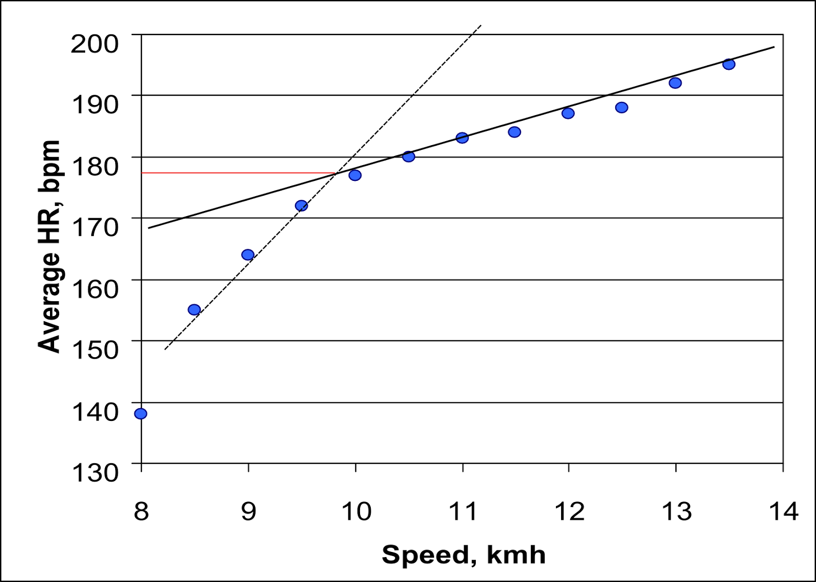
This behavior is not observed by all athletes¹. But, it is judicious to take it into account in a modeling.

Indeed, an affine model will be imprecise if this situation happens. The following simulation illustrate it:

If the runner does all his runs below the deflection point, we will have a model quite close to reality. But, as soon as he run at high intensity, he disturbs the model and it will no longer be correct enough neither below the aerobic threshold, nor above.

The solution is to add a function that adds a curvature. Here is a simple example that gives good results:

$$ HR = a + b \times Power + c \times \log(Power + 1) $$

a, b and c are the parameters to be determined by analyzing the data.

Here is, on the same simulation example, we can see the behaviour of this model:

We see that the model follows the reference curve much better even if it is very primitive.

More general modeling

Using power over an interval is not generic enough. That supposes that the interval is long enough for stabilizing the heart rate. This is an assumption that may be valid for a protocol like the Conconi or the Cooper test. But, for being valid for any run, it is necessary to use a more generic model.

The idea is to reuse the same model and apply it to the power averages over different durations: the power of the 15 last seconds, last 30 seconds and so on.

The formula is then:

$$ HR = a_0 + \sum_{i=1}^{5}{ a_{3i-1} \times P[-15i\ldots 0] + a_{3i-2} \times \log( P[-15i\ldots 0] + 1 ) } + a_{3i} \times D[-15i\ldots 0] $$

P[a…b] is the average power of the relative moment a until the moment b. P[-7…0], P[-14…0] and P[-28…0] are the average power of the Last 7, 14 and 28 seconds. D[a…b] is the standard deviation of the interval [a…b]. We use for our model the measurements over 15s, 30s, 1 minute, 2 minutes and 4 minute The parameters a0 to a16 are determined to minimize the error between the measured heart rate and the estimation.

This formula has the advantage of not making any assumptions about the athlete’s form. For an occasional runner, the recovery is often longer and therefore the physical effort of the previous minutes has more effect than for an athlete.

However, this assumes that the heart rate can be determined on rather brief moments. It is therefore not adisable to use a wrist-based sensor. Besides the fact that they often produce values completely wrong when they are badly positioned, they tend to average heart rate over several tens of seconds. The chest strap monitor should be preferred (do not forget to humidify the contacts²)

Then, we should keep in mind that we have here a machine learning algorithm. It is only able to predict what it already learned! That’s why it is theoretically necessary to run the full range of the runner’s power possibilities, for long and short time frames. It is obviously not possible to do this during a single session. This is the reason why it is necessary to run several hours before to get an acceptable precision. Generally saying, after having only done series of slow run sessions, the algorithm will be unable to deduce the frequency during a real race runt at the maximum of the athlete’s capabilities. It will produce first wrong predictions and gradually adjust by learning this new configuration.

Real Environment tests

To test the algorithm it is first necessary to do calibration sessions which permits learning the correspondence between heart rate and power. It is illusory to think obtaining a significant result after one or two short runs.

For all sessions, I measure the difference between the estimated heart rate and the measured heart rate. A zero value means that the estimation is perfect. A positive value means that the measured heart rate is lower than estimated (+3 means I saved 3 beats per compared to what was expected). To facilitate comparison, all curves display the same data:

• The measured heart rate (gray curve)
• Power (yellow curve)
• The difference between heart rates (red curve)

Learning sessions

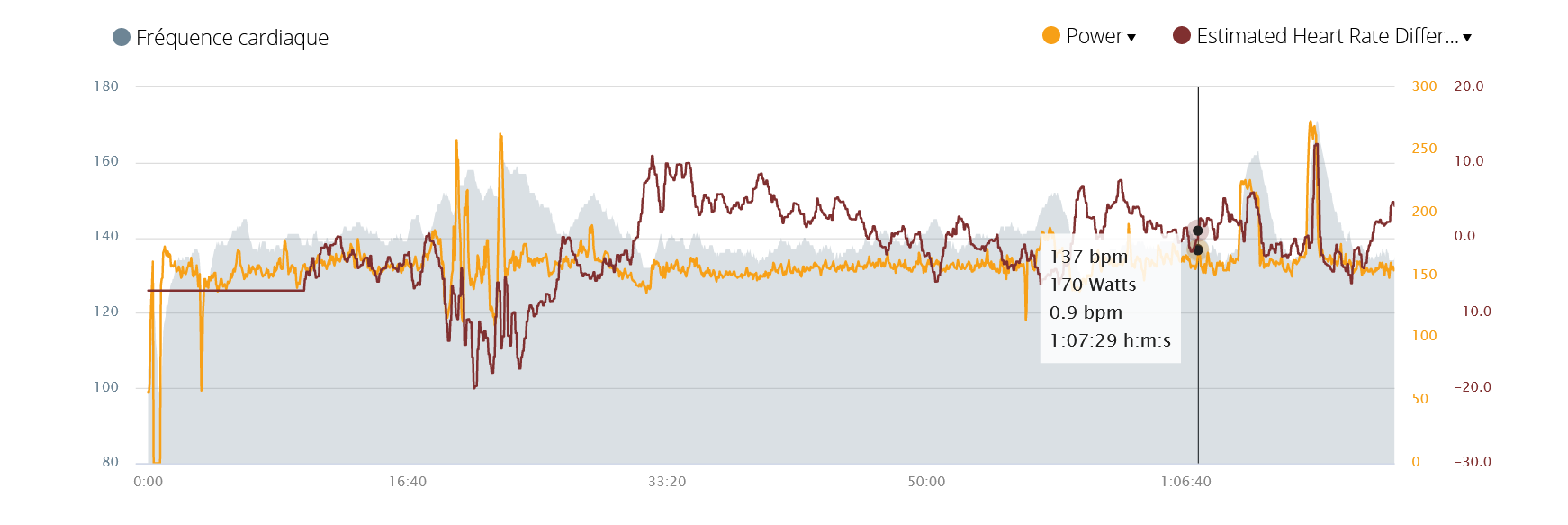
First session: moderate run

The first results needs to be taken with care because the algorithm may lean by heart the correspondence. One of the signs is that the first guess at the beginning of the run had no error:

The precision of algorithm then tends to oscillate because all the measurement errors of the Stryd sensor and the heart rate monitor tend to influence the result. But, we remain with a good average error around 2 pulsations.

However, it is too early to start interpreting the results because this session was a slow run with some variations in speed but no intervals, no hills, no farlek…

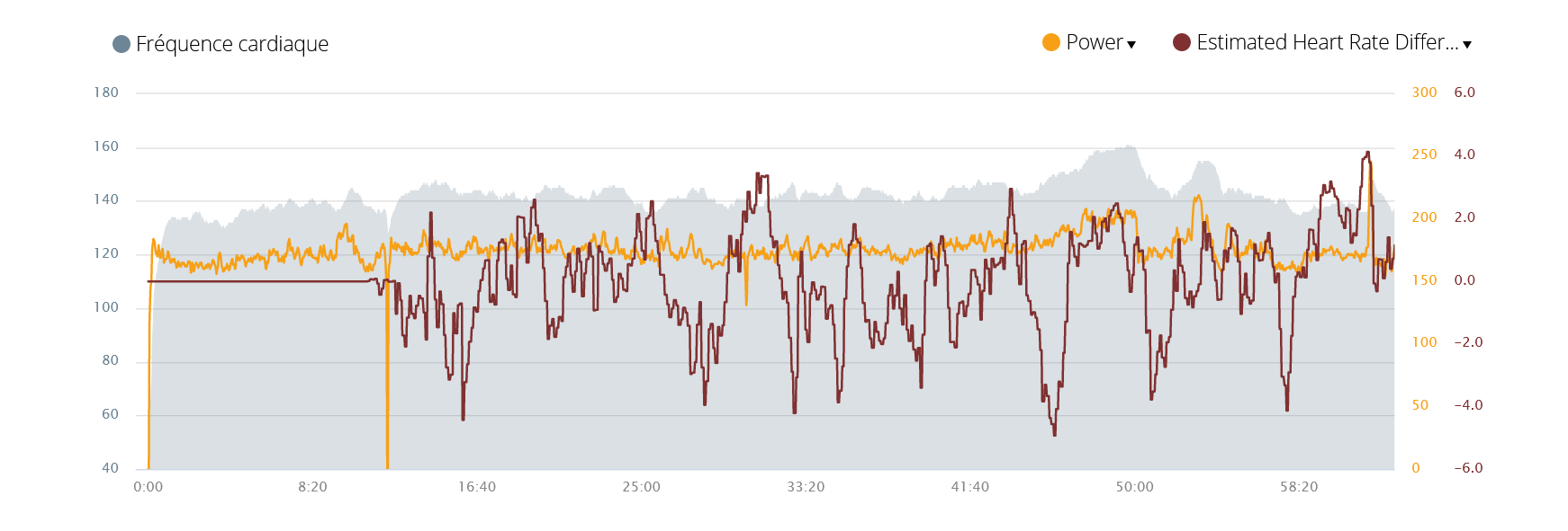
Second session: slow running with a few accelerators

For a second run, I decide to run more slowly and to use a small portion of a very irregular cross-country road between the 16th and 25th minute:

I chose this portion because it is particularly difficult to estimate the power. Indeed, this path is composed of steep hills with a height of 10m maximum with a slope impossible to climb without good run-up. A lot of obstacles, which require to pay attention, are on this path and it is difficult to maintain his rhythm.
The Stryd sensor does not deliver anything convincing in this situation. It needs 3-4 seconds to estimate a power and, if the effort is not stable, the power is poorly estimated. In addition, the nature of the terrain here generates an additional effort which is not alone measurable in the legs but which is fully reflected on the heart rate. The result is that the power remains more or less stable (apart from a few peaks) but the heart rate increases independently to the power.

The algorithm, with only one hour of running learned, has not enough data to handle correctly this situation and is influenced by this portion. We see that the estimation was up to 20 beats higher as measured. Then, once we leave this area, the algorithm underestimates by 10 beats the heart rate and gradually relearn steps by step the correlation between the power and the heart rate. After 30 minutes, the algorithm gives again a good heart rate estimation. This test clearly shows the stability of the algorithm: after 1 hour of learning, an atypical portion of 10 minutes can certainly influence it but it corrects it very quickly with a few extra minutes of running in a normal constellation. It is clear that with several hours of running sessions in memory the influence of such a portion will be negligible.

Finally, I accelerated a few times. Again, same problem, the algorithm has never dealt with such high power in a short time frame. That’s why the heart rate estimated is not yet reliable for this exercise.

First intervals

After 3 learning sessions with more or less regular races, I decides to do 30s intervals with 30 seconds of recovery. The sudden variations of intensity have not yet been learned. Therefore it does not wonder that we will get significant estimation errors:

In the first phase of the run, which is a moderate warm-up, the prediction remains good. It is also interesting to note that the power seems to be more or less constant but the heart rate drifts slowly. The algorithm detects this because the difference between the measured heart rate and estimated gradually changes from +5 beats to -5 beats. Maybe a decrease of my physical fitness? I can not remember anymore.

The first intervals are very poorly predicted because it does not really predict the increase in heart rate (difference of -10 pulsations). But, it is quickly corrected on the next intervals and the frequency predicted is then closer to reality. (with a difference between 0 and +5 pulsations) The recovery phase is also new and not really taken into account. It will take more races to correct this point.

In any case, we can clearly see that we must teach running situations to the algorithm. There is no reliable prediction of an new context.

Results

The first really significant results are obtained after 5 or 6 hours of running. Before, the algorithm is not reliable because in the first few minutes, it learns the configurations by heart and then, it does not have enough data to ensure a statistical robustness.

Here are some typical races and the records obtained.

Running in good shape

There are such days where everything is perfect: the weather is nice and you’re really feeling fit. Just after starting to run, as I look at the watch, I was amazed to be so fast. However, I did not have the impression of make a significant effort. This is the kind of situation reflected in the following recording:

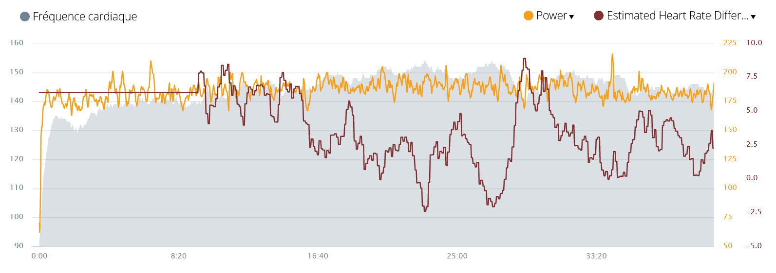
I was already a little surprised when I took a look at my watch, the frequency heart rate seemed lower than usual. But I took that this could only be an impression. It is clear that by looking from time to time at his watch, this moment does not necessarily reflect a reality over an entire race. And then, was I not not the victim of an analysis distorted by my optimism of this day?

That said, the offline analysis showed that my heart rate was systematically lower with an average of 4 to 5 beats. What is remarkable is that the Garmin algorithm that determines the performance condition gives the same result³:

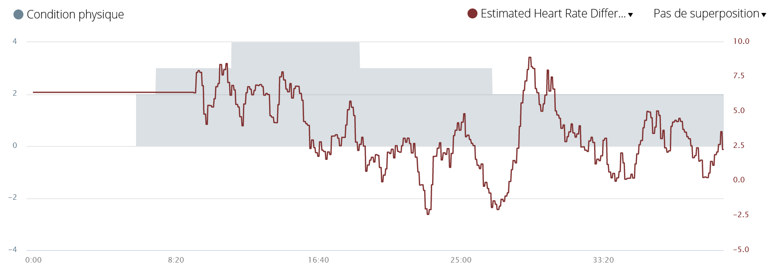
However, the correlation between heart rate and current fitness may just be a coincidence. This point should be confirmed by scientific papers and by a more in-depth long-term test.

Trail

After ten hours of running in the plains, I decided to test it on trail. It was a track not too steep and, therefore, there was no need to resort to walking. Since I ran during 5 continuous days, I did not expect a lower heart rate for a given power. Short-term fatigue tends to cause a small drop in shape. And, anyway, the effort with trail running is greater than with running on the road: it is necessary to pay much more attention to the roughness of the paths, to avoid potholes, stepping over obstacles … the rhythm is less regular. As result, we pay a price in terms of energy expense and therefore, on the heart rate.

For this session, the heart rate was approximately 5 beats higher than usual, this is consistent with the measured difference (constantly negative and around -5). Nevertheless, for this session, a new configuration appeared: at the crossroads, we took a break to wait for the whole group. It’s a situation not yet taken into account by the algorithm: the power was falling to be zero for several minutes.

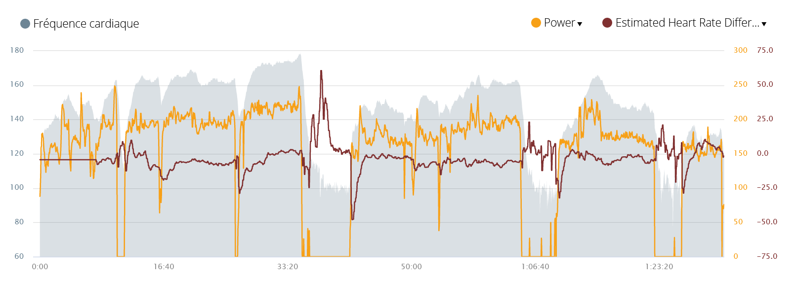
As can be seen during the first stop, the heart rate estimated is completely disconnected from reality. It is even up to 50 pulsations lower than the measurement! On the other hand, this bad estimate is corrected from the second break with a more modest difference that does not exceed 15 beats.

I must recognized that this is an extremely difficult situation to predict. This is equivalent to estimating the recovery time. But, everyone knows that this can vary enormously from one day to another. Here it is even more complicated: a null power value can certainly correspond to a recovery but not necessary. It is not because we do not walking that we do not move our arms, discuss, stay calm… In short, we are here in a borderline case where the algorithm does not does not really apply. On the other hand, it is remarkable that it is still learning it after many hours of runs in memory and corrects the error during the next pause.

Hill intervals

Finally, I decided to do a test with intervals on hills. The 30/30 intervals were already learned during a previous session but here, I decided to do it on a slope of 10%.

First of all, it must be said that power is really an asset here: the speed when climbing a hill with high intensity is comparable to the speed of a slow run on the flat. It would therefore be impossible for an algorithm to predict the heart rate frequency by analyzing only the paces. Here, the power makes it possible to deal with this situation.

Nevertheless, the intervals of 25s made here are at the limit of what can be analyzed:

• Stryd sensor only delivers power information after 3 to 4 seconds, the acceleration phase cannot really be analyzed.
• The chest belt itself has a similar latency, which poses a problem to learning part of the algorithm
• Then, the algorithm analyzes the data every 7 seconds, and it is possible that the heart rate estimation is made at the moment where the sensors provide unreliable values.

The algorithm had already repeatedly learned the behavior during 15s, 30s and hill intervals. So there is no reason why it should deliver crazy results.

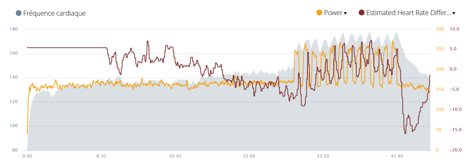
Here is the variation of the difference between the estimated and the measured heart rate:

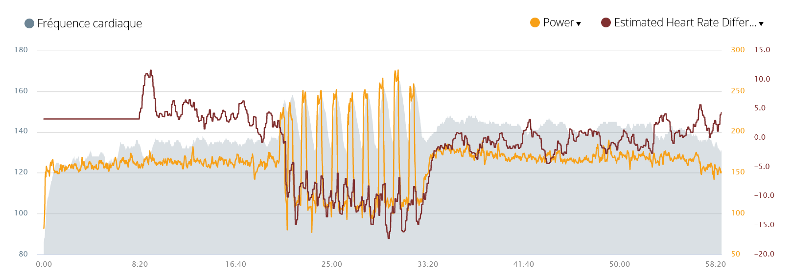
We can see 4 stages:

1. the first 10 minutes: no estimation is made during the warm-up.
2. a first very slow run, quite easy and giving me the impression of having been in great shape. The estimated heart rate is 3-4 beats higher than the measured one.
3. the 25s intervals on a hill: there the estimation is 10 to 13 beats higher than what was estimated. It may be a bit exaggerated but it is quite consistent with my feeling because I had the impression that it was difficult exercise (it’s not surprising because I had run too much during the previous days).
4. For the rest of the run, the estimated heart rate is about the same as the measured one. It’s pretty consistent with what I felt: these intervals exhausted me a bit. If I compare with the start of the race, which was easier, it’s normal that my heart rate is a little higher for the same effort.

Conclusion

I can say that after two good weeks of running, I get quite interesting results. After few calibration runs, I can compare the evolution of the heart rate from session to session or follow the evolution during a session. It opens some opportunities for a follow-up of the fitness over few weeks. But, I must admit that, due to my lack the knowledge of sports medicine, I cannot make a statement on this.

Anyway, the produced result remains easily interpretable: we get the heart rate difference in comparison to what was learned to the previous sessions. A coach who is used to work with the heart rate should not be confused. It is less complicated to interpret as for the power which differs from athletes to athletes.

In all cases, the results are interesting enough to develop new features for Garmin watches:

• Calculation of heart rate zones from power zones (or vice versa)
• A calculator that can predict track speed, power and heart rate for long runs.
• Real-time information of the heart rate drift during the session.